Symmetry Factorization of Lamé Equation

Idiong U.S.¹

¹Adeyemi Federal University of Education, Ondo State, Nigeria

*Corresponding Author Email: usidiong@gmail.com …

Read More

Highlights

Abstract

The study of Lamé operator remains an open problem because of its rich symmetry and other algebraic properties. One of the essential tools that is used in its study is the factorization technique. This paper gives some of the answers to the questions that arise in the consideration of the integration of the Lamé operator equation on the elliptic curve using infinitesimal transformation.

Keywords: Elliptic, Factorisation, Infinitesimal transformation, Lie symmetry, Lame equation.

1. Introduction

Lam´e equation in its different forms are second order ordinary differential equations in the complex domain. They appear in literatures as Fuchsian differential equations with four regular singularities e1​=℘(ω1​), e2​=℘(ω2​), e3=℘(ω3), and e4=∞, where ω2=(ω1+ω3)/2 (see Churchill, 1989). In its compact Weierstrass form

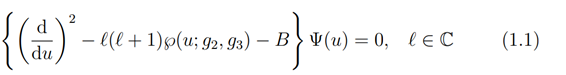
is defined on the family of elliptic curve

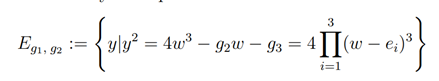
where B is the accessory parameter which plays the role of the eigenvalue of equation (1.1) and ℘(u) is the Weierstrass elliptic ℘-function. In the selfadjoint Fuchsian form

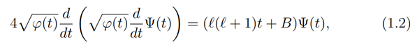
where, φ(t)=(a ²+t)(b²+t)(c ²+t)=(℘(u)-e1)(℘(u)-e2)(℘(u)-e3)=(a ²-b ²)² sn ² α cn²α dn²α, and (a ²-b ²) ² ∈R (see Wang et. al 1989, pp. 576- 580, §11.1). Here, t can assume any variable λ, µ, ν in the coordinates of the ellipsoid.

The major existing technique for solving the Lam´e equation is the operator factorization which gives elliptic solutions. The Ricatti equation plays an intermediary role in the study of Supersymmetry (SUSY) factorization as well as Lie symmetry analysis of Schr¨odinger operators. Hence, the need to understand a technique of solving Riccati equation and its Lie symmetry considerations cannot be overemphasized. The paper shall be outlined as follows: section 2 deals with infinitesimal transformation and the solution of Ricatti equations; section 3 deals with the Lie symmetry of Ricatti equations and section 4 deals with our main results.

2. Infinitesimal Transformation and the Solution of Ricatti Equations

In this section, we examine the group theoretical approach of solving ordinary differential equations using infinitesimal transformations.

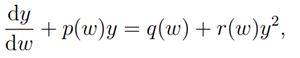
2.1 Theorem (Hill 1992, p. 31). Consider the generalized Riccati equation

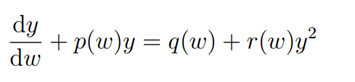
which remains invariant under the transformation of the form

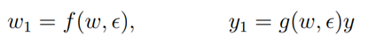
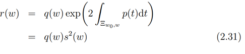
provided r(w)=q(w)s(w)². Then the infinitesimal displacement functions

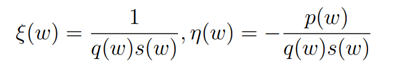
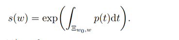
with suitable canonical coordinates

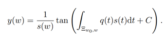
reduces the Ricatti differential equation to a solvable form

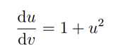
so that the solution of the Ricatti differential equation is

Proof. Now, given the generalized Ricatti equation

let

By one-parameter group infinitesimal transformation

Taking the derivative of equation (2.2) we have

Now taking the quotients of parametric derivatives in (2.3) we obtain by first prolongation formula (see Gilmore, 2008,§16.2.2, p.287)

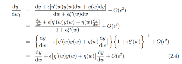
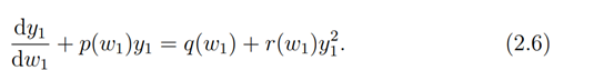
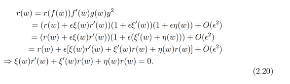
as ϵ². Next, we show that the generalized Ricatti equation

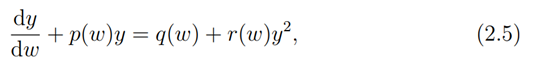
remains invariant under the transformation (2.5) provided r(w) = q(w)s(w) ² i.e.

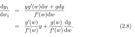
Now, from (2.5) we have

so that taking the differential quotient we have

Now, substituting (2.5) and (2.8) into (2.6), we have

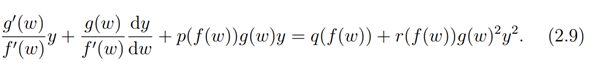
Multiplying through (2.9) by (f'(w))/(g(w)), we obtain

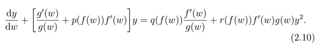
Now, comparing (2.5) with (2.10) we have

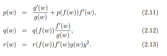
Now setting,

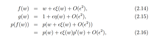
and similarly,

Thus from (2.11)-(2.17) we have

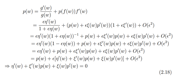
and

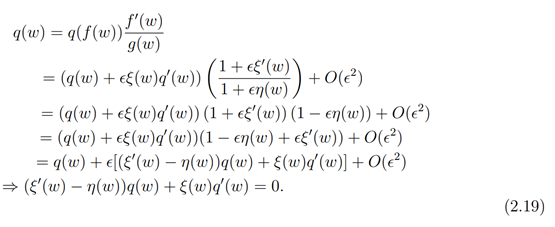
Also,

Now equations (2.11)-(2.13) can now be rewritten respectively as

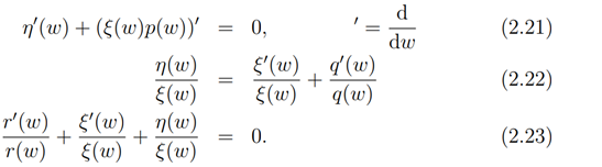
Substituting (2.22) in (2.23) we have

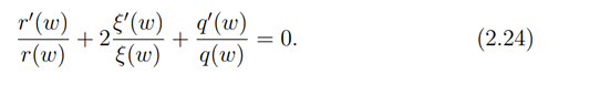
Integrating (2.24) we have

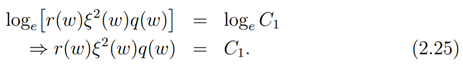
Also integrating (2.21) we obtain

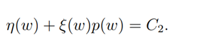
Now, let C₂ = 0, then we have that

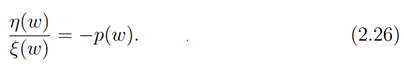
Substituting (2.26) into (2.22) it is easily seen that we have

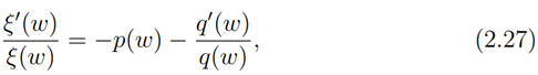
which on integrating gives us

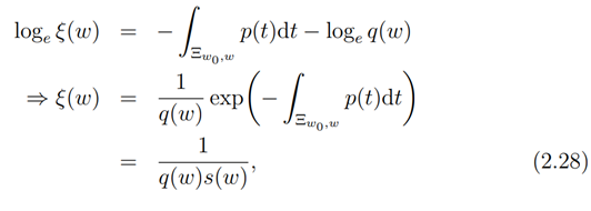
where

Now from (2.26) and (2.28) we have

Furthermore, substituting (2.27) into (2.24) we have

On integrating (2.30) we arrive

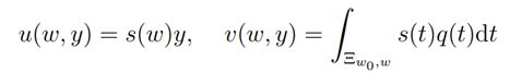
 If we now choose our canonical coordinates to be

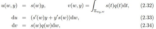
so that taking the quotient of (2.33) by (2.34)

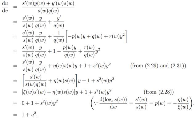
By variable separable method we have

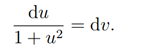
Integrating both sides, we have

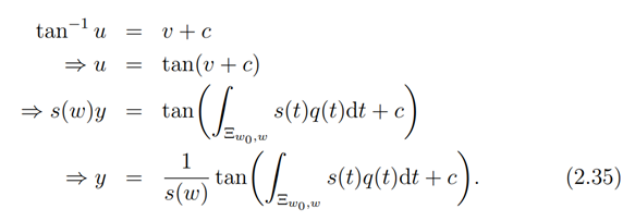
The result is obtained as required.

The result is obtained as required.

The above result holds where w,w_o ∈C∖{0,∞}are two endpoints which are connected by a simple rectifiable curve Ξ(w_o​,w)​.

3. Lie Symmetries

In this section, we discuss the Lie symmetries of differential operators which is an important tool for the study of the group properties of a linear differential operator. We know (Cariñena & Ramos, 1998, p.3) that Ricatti equation of the form

can be considered as a differential equation determining the integral curves of w-dependent vector fields

so that X_ω is the linear combination with ω-dependent coefficients of the three vector fields

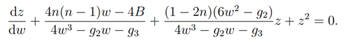
Now the Riccati equation associated to Brioschi-Halphen equation (BHE)

can be obtained by setting

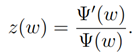
Thus, the associated Riccati equation is given by

Here, z=z(w).. This implies that the differential equation determining the integral curves of w-dependent vector fields can be written as

Now let a₁(w),a₂(w),a₃(w) be functions related to the family elliptic curves E_g2,g3 which are expressed by

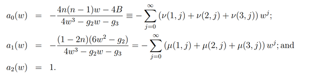
Here,

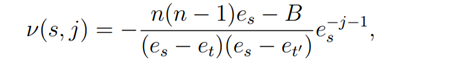
and

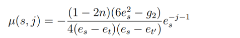
where s,t,t^’=1,2,3,s≠t and s≠ t^’

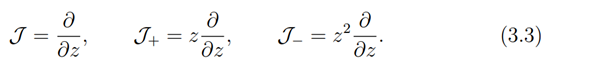
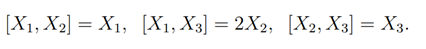
The basis of the vector fields Xω made up of {J,J+​,J−​} are the generators of a Vessiot-Guldberg Lie algebra, ⟨J,J+​,J−​⟩ ≅ sl(2,C) , which is made up of traceless matrices having basis

with Lie algebraic commutation

We remark here that the matrices H, E+, E− in (3.6) commute exactly as theJ,J+​,J− in (3.3). It is also observed that J, and J+​ generate a 2-dimensional Lie subalgebra isomorphic to the Lie algebra of the affine group of transformation in one dimension and same holds for J+ and  J−. The one parameter subgroups of local transformation of C generated by J,J+ and J− are respectively

• Translation ω↦ω+ϵ
• Dilation ω↦e^(ϵ)
• Infinitesimal/Mobios ω↦ω/(1-ωϵ)

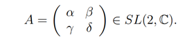
for which+J_(- )is not a complete vector field of C. However, a one point compactification of C is practicable and then J,〖 J〗_(+ )and J, could be considered as the fundamental vector fields corresponding to the action of SL (2,C) on the complete complex rectifiable curve. CP^1=C∪{∞} given by

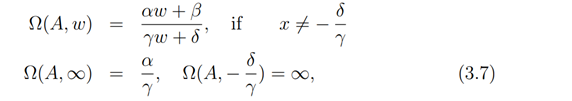
where,

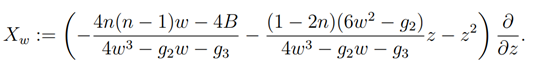
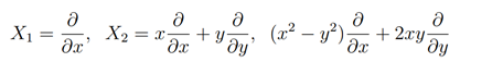
Alternatively, the vector field Xw in (3.2) can also be written as

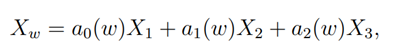
where

which also span the Vessiot-Guldberg Lie algebra of vector fields V≃ sl(2,C) which obeys the commutation relation

Hence, {Xω}_ω∈CP¹ ⊆ VX ⊆ V and V^x is finite-dimensional, which makes X into a Lie system. Hence, it admits a superposition rule. This is an analogy to what is obtained in (Munoz, 2015).

4. Main Result

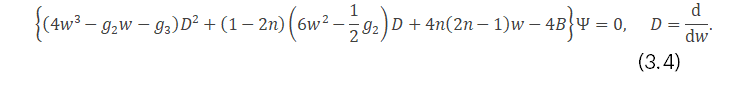
Next, we compute the eigenfunctions of the Lam´e equation using the infinitesimal transformation of its associated Riccati equation. Now having obtained a quadrature (2.35) we now apply it to factorization of the Lamé operator equation. The Lamé equation obtained from ellipsoidal harmonics, takes the form

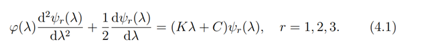
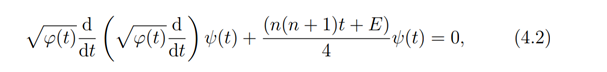
Here φ(t)=(a² +λ)(b² +λ)(c²+λ)=(℘(u)-e₁)(℘(u)-e₁)(℘(u)-e₃)=(a²-b²)² sn²αcn²αdn²α, K=n(n+1) and (a²-b²)²∈R. If without loss of generality we set ψr ≡ ψ and the Lam´e operator equation (4.1) in self adjoint form takes the form

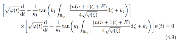
Proposition 4.1

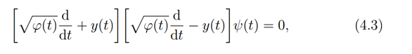
The Lamé equation (4.1) factors as

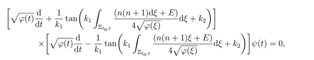
having the eigenfunctions

Proof. Let the equation (4.2) factor as

which on multiplying out gives us

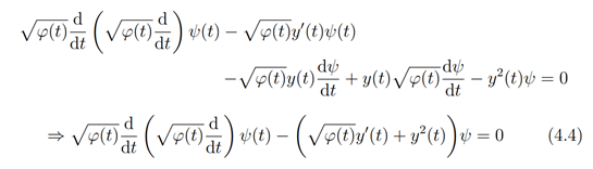
Now comparing (4.2) with (4.4) we have

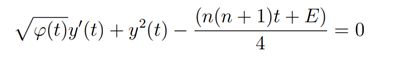
which can be rewritten as

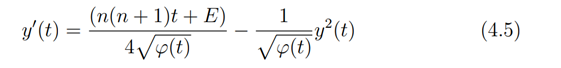
Comparing (4.5) with the generalized Riccati equation in (2.5) we obtain

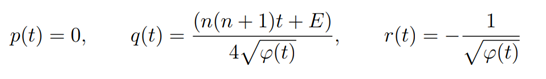
so that,

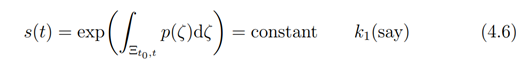
From (2.35) we have

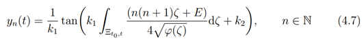
(4.7) holds for the case t = λ, ν. For the case t = µ we replace φ(t) with −φ(t), we have

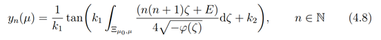
where (4.7) and (4.8) gives us the super potential for the operator (4.2) So that (4.3) now becomes

Now, the eigenfunctions ψ≡ψ_n^((-)) (t,E)are obtained by solving the 1st order linear differential equation

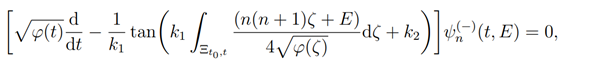
which can be rewritten in the form

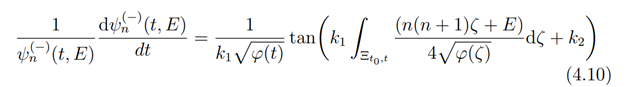
Now, we integrate both sides of (4.10) to obtain

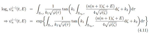
where, τ∈[0,t]. Similarly, the eigenfunctions ψ_n^((+))which satisfy the 1st order linear operator equation

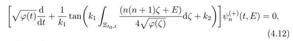
are obtained as

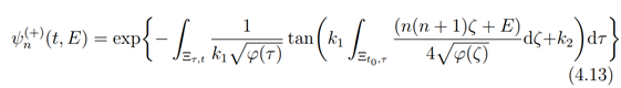
In the cases (4.11) and (4.13), t = λ, ν, analogously we obtain the eigenfunctions in terms of t = µ by replacing φ(t) by −φ(t) for which we obtain hyperbolic trigonometric solutions. In each case we obtain a sequence of eigenfunctions {ψ_n^(-)(t,E)}, {ψ_n⁽⁺⁾(t,E)}∈H_t,t=λ,μ,ν with n ∈ N. The sequence generated allow for consideration of completeness of the Hilbert space.

5. Conclusion

The result obtained in this paper shows a new alternative technique of solving second order differential equations and in particular the Lamé equation through a proper understanding of Lie symmetries and infinitesimal transformation.

Conflict of Interest

The research was completed with no conflict of interest.

References

Cariñena, J.F. and Ramos A. (1998). Integrability of Riccati equation from a group theoretical viewpoint. arXiv:math-ph/9810005v1

Churchill R.C. (1989). Two Generator Subgroups of SL(2,C) and the Hypergeometric, Riemann, and Lame Equations. J. Symbolic Computation 28(1999)521-545.

Gilmore R. (2008). Lie Groups, Physics and Geometry-An Introduction to Physicists, Engineers and Chemists. Cambridge University Press. 2008

Hill, J.M. (1992) Differential Equations and Group Methods for Scientists and Engineers. CRC Press. Tokyo.

Munoz, C.S. (2015) Lie Systems, Lie Symmetries And Reciprocal Transformations.Ph.D. Thesis. arXiv:1508.00726v1 [math-ph]

Wang Z.X., Guo D.R. and Xia X. J. 1989. Special Functions. World Scientific Publishing Co. Plc. Ltd. Singapore.

About this Article

Cite this Article

APA

Idiong U.S. (2024). ASymmetry Factorization of Lamé Equation. In K. S. Adegbie, A. A. Akinsemolu, & B. N. Akintewe (Eds.), Exploring STEM frontiers: A festschrift in honour of Dr. F. O. Balogun. SustainE.

Chicago

Idiong U.S. 2024. “Symmetry Factorization of Lamé Equation.” In Exploring STEM Frontiers: A Festschrift in Honour of Dr. F.O. Balogun, edited by Adegbie K.S., Akinsemolu A.A., and Akintewe B.N., SustainE.

Corresponding Author Email: adisaio@aceondo.edu.ng

Disclaimer: The opinions and statements expressed in this article are the authors’ sole responsibility and do not necessarily reflect the viewpoints of their affiliated organizations, the publisher, the hosted journal, the editors, or the reviewers. Furthermore, any product evaluated in this article or claims made by its manufacturer are not guaranteed or endorsed by the publisher.

Distributed under Creative Commons CC-BY 4.0

Share this article

Use the buttons below to share the article on desired platforms.